Article Text

Abstract
Study objective: In social epidemiology, it is easy to compute and interpret measures of variation in multilevel linear regression, but technical difficulties exist in the case of logistic regression. The aim of this study was to present measures of variation appropriate for the logistic case in a didactic rather than a mathematical way.
Design and participants: Data were used from the health survey conducted in 2000 in the county of Scania, Sweden, that comprised 10 723 persons aged 18–80 years living in 60 areas. Conducting multilevel logistic regression different techniques were applied to investigate whether the individual propensity to consult private physicians was statistically dependent on the area of residence (that is, intraclass correlation (ICC), median odds ratio (MOR)), the 80% interval odds ratio (IOR-80), and the sorting out index).
Results: The MOR provided more interpretable information than the ICC on the relevance of the residential area for understanding the individual propensity of consulting private physicians. The MOR showed that the unexplained heterogeneity between areas was of greater relevance than the individual variables considered in the analysis (age, sex, and education) for understanding the individual propensity of visiting private physicians. Residing in a high education area increased the probability of visiting a private physician. However, the IOR showed that the unexplained variability between areas did not allow to clearly distinguishing low from high propensity areas with the area educational level. The sorting out index was equal to 82%.
Conclusion: Measures of variation in logistic regression should be promoted in social epidemiological and public health research as efficient means of quantifying the importance of the context of residence for understanding disparities in health and health related behaviour.
- logistic regession
- mulilevel analysis
- social epidemiology
Statistics from Altmetric.com
In the study of contextual determinants of health, considering the extent to which individual health phenomena cluster within areas is not only necessary for obtaining correct estimates in regression analysis. It also provides relevant information that permits assessment of the importance that the context has for different individual health outcomes.1,2
In multilevel linear regression analysis it is easy to partition the variance between different levels and compute measures of clustering that provide intuitive information for capturing contextual phenomena.3–5 However, for binary outcomes, the partition of variance between different levels does not have the intuitive interpretation of the linear model. Despite these difficulties several methods have been developed in logistic regression to obtain suitable epidemiological information on area level variance and clustering within areas.6–9
This paper represents the last of a series of four included in a project aimed to explain in a conceptual rather than a mathematical way how to calculate and interpret multilevel measures of variance and clustering.3–5 This study is focused at measures of variation in logistic regression. We put a special emphasis on indicating the relevance of these measures in social epidemiology and community health.1
THE ILLUSTRATIVE EXAMPLE
Background and objectives
In Sweden individual economic resources are not an important determinant for choosing private compared with public healthcare practitioners as the county council supports patient fees in both cases. The choice of a private rather than a public practitioner may express individual preferences, demands, and expectations related to socioeconomic position. Moreover, place of residence may influence this individual decision over and above individual characteristics. In this study, we used multilevel measures of variance and clustering to quantify the contextual dimension of this healthcare seeking behaviour.
Population and methods
Data sources and variables
Our illustrative analysis was based on the health survey in Scania conducted in 2000, a postal self administered questionnaire survey.10 Each of the 33 municipalities of the county of Scania, Sweden, corresponded to a survey area, except the four largest municipalities Helsingborg, Kristianstad, Lund, and Malmö, which were subdivided into 6, 5, 10, and 10 administrative areas respectively. In total there were 60 different survey areas. The initial survey sample consisted of 23 437 persons born between 1919 and 1981, 13 715 (59%) of whom agreed to participate. The survey seems largely representative of the total Scanian population. An important concern, however, is the under-representation of the immigrant population.11
After approval by the ethical committee at the Medical Faculty of Lund, survey data were linked to the 1999 patient administrative register, which contains individual level information on utilisation of all public and private health care financed by the county council in Skåne. This study only considered people who had had at least one contact with a health care provider during 1999 (10 723 persons aged 18–80 years).
The binary outcome distinguished those persons who had consulted a private physician at least once in 1999 from those who had not. Age was introduced as a continuous variable. Sex (men v women) and educational level (nine years or less, more than nine years) were divided into two categories. An area level socioeconomic variable, defined as the percentage of highly educated inhabitants, was coded in two classes with the median value as the cut off. This area variable was derived from data on the whole population of the county.
Multilevel analysis
We aimed to investigate whether the residential area determined the choice of a private as compared with public practitioner. We first estimated an “empty” model (model i), which only includes a random intercept and allowed us to detect the existence of a possible contextual dimension for this phenomenon.3 Thereafter, we included the individual characteristics in the model (model ii) to investigate the extent to which area level differences were explained by the individual composition of the areas.4 Finally we added the area variable (model iii) to investigate whether this contextual phenomenon was conditioned by specific area characteristics.5
The multilevel logistic regression models were estimated with Markov Chain Monte Carlo (MCMC) method using MLwiN software (version 1.2) developed by Goldstein research group.12,13
THE MULTILEVEL LOGISTIC REGRESSION
In logistic regression the aim is to predict the probability pi that a phenomenon (for example, visiting a private physician) occurs for the individual i in function of a certain number of variables. As the natural values of pi extend from 0 to 1 and a regression analysis is better performed on values between −∞ and +∞ we transform pi in logit (pi), which is comprised of values between −∞ and +∞.14
More specifically, multilevel logistic regression considers that the individual probability is also statistically dependent on the area of residence of the subjects. This dependence on the context needs to be accounted for to obtain correct regression estimates, but doing so also conveys substantive information in itself.1,15,16
In model i (the empty model) the probability of visiting a private physician is only function of the area in which the people live, which is accounted for with an area level random intercept:

M = overall mean probability (prevalence) expressed on the logistic scale
EA = area level residual*. The area level residuals are on the logistic scale and normally distributed with mean 0 and variance VA.
VA = area residual variance expressed on the logistic scale (that is, variance around M)
VI = pi (1 – pi) = individual variance expressed on the probability scale, and depending on the predicted probability pi of the outcome.
In model i the probability of visiting a private physician for a person living in an area A depends on M and EA. Equation 1 can be rewritten as

In model ii the probability of visiting a private physician is function of the area of residence of the people and of the individual variables (sex, age, and education).

β1, β2, β3 = regression coefficients for the individual covariates
In model iii the probability of visiting a private physician depends on the residential area of the individuals, on the individual variables, and on the area educational variable.

β4 = regression coefficient for the area level educational variable
MEASURES OF AREA LEVEL VARIANCE AND CLUSTERING IN MULTILEVEL LOGISTIC REGRESSION
Intraclass correlation and the related variance partition coefficient
We have previously discussed the relevance of the intraclass correlation coefficient (ICC) (also termed variance partition coefficient (VPC) in its most general form) for understanding contextual phenomena expressed with continuous variables.3–5 In the linear case, the ICC informs us on the proportion of total variance in the outcome that is attributable to the area level.

where VA is the area level variance and VI corresponds to individual level variance.
In the linear model, the ICC is based on the clear distinction that exists between the individual level variance and the area level variance. Indeed, knowing the mean value of a continuous outcome variable in each area, you would not be able to infer the values of the variable for each individual: the individual level variance within areas could be small or very large. By contrast, with a binary variable the individual level values (0 and 1) are apparently known from the prevalence existing in each area. This absence of a clear distinction between individual level variance and area level variance makes it trickier to compute and interpret the ICC in logistic models.
In multilevel linear regression both the individual level and the area level variances are expressed on the same scale (for example, mm Hg for systolic blood pressure). Therefore, partition of variance between different levels is easy to perform for detecting contextual phenomena.3–5 In multilevel logistic regression, however, the individual level variance and the area level variance are not directly comparable. Whereas the area level residual variance VA is on the logistic scale, the individual level residual variance VI is on the probability scale. Moreover, VI is equal to pi (1 – pi) and therefore depends on the prevalence of the outcome (that is, the probability).
To solve these technical difficulties, Goldstein and others6,17 have described some alternative approaches for computing the ICC in the case of logistic regression. Two of these methods are (a) the simulation method6,7; and (b) the linear threshold model method, or latent variable method supported by Snijders and Bosker.17 Both methods convert the individual level and area level components of the variance to the same scale before computing the ICC.
(a) The principle of the simulation method is to translate the area level variance from the logistic to the probability scale in order to have both components of variance on the probability scale. These two components of variance can then be used on the probability scale to compute the ICC with the usual formula (equation 5). More details on this approach are provided in table 1 and elsewhere.6,7
Hypothetical data showing that the size of the intraclass correlation (ICC) calculated by the simulation method6 in a multilevel logistic model depends of the prevalence of the outcome (that is, the predicted probability). We present 11 cases, all with the same area variance VA but with different outcome prevalence (pI)
As noted previously, the individual level variance depends on the prevalence. A first consequence is that different phenomena with a similar area level variance but a different prevalence (M) will have different ICCs. As illustrated in table 1 using hypothetical data, for a given amount of area level variation, the ICC will always be the highest for outcomes with a prevalence of 50%. This aspect needs to be considered when comparing the magnitude of clustering between phenomena with a different prevalence.
A second consequence occurs in the model including covariates. As the ICC depends on the prevalence, which in turn depends on the characteristics of the individuals, there will be one different ICC for each different type of individual. Note that this heterogeneity in the ICC is just a consequence of the dependence of this definition of the ICC on the prevalence of the outcome.
(b) The linear threshold model method or latent variable method converts the individual level variance from the probability scale to the logistic scale, on which the area level variance is expressed. In our case, the method assumes that the propensity for visiting a private physician is a continuous latent variable underlying our binary response (that is, having visited a private physician or not). In other words, every person has a certain propensity for visiting a private physician but only persons whose propensity crosses a certain threshold actually do it. The unobserved individual variable follows a logistic distribution with individual level variance VI equal to π2/3 (that is, 3.29).6,7,17 On this basis, the ICC is calculated as:

The ICC is only a function of the area level variance and does not directly depend on the prevalence of the outcome as in the simulation method.
These methods for computing the ICC in logistic models have their own statistical consistency. However, they are an attempt to apply to the logistic case notions that are based on the clear distinction between the individual level variance and the area level variance that exists in the linear case. As this distinction is not so clear in the logistic case, the interpretation of the ICC for dichotomous outcomes is difficult to understand in epidemiological terms.6,8,18
The median odds ratio
The aim of the median odds ratio (MOR)8,9 is to translate the area level variance in the widely used odds ratio (OR) scale, which has a consistent and intuitive interpretation. The MOR is defined as the median value of the odds ratio between the area at highest risk and the area at lowest risk when randomly picking out two areas the MOR can be conceptualised as the increased risk that (in median) would have if moving to another area with a higher risk. In this study, the MOR shows the extent to which the individual probability of visiting a private physician is determined by residential area and is therefore appropriate for quantifying contextual phenomena. The MOR is statistically independent of the prevalence of the phenomenon, and can be easily computed in the empty model and in more elaborated models.
To intuitively understand the rationale for the MOR, imagine that we consider all possible pairs of persons with similar covariates but residing in different areas. In figure 1 we consider two different fictive cases, one with weak variations between areas, the other with very strong variations. Using the area level residuals of the multilevel model we compute the OR for each pair of persons with the subject with the higher odds always placed in the numerator (the OR is always larger than or equal to one). This procedure yields a distribution of the OR. Figure 2 gives the distribution of the OR that we obtained in considering the 56 million pairs of persons from different areas that can be formed in our dataset. The MOR is the median of this distribution.
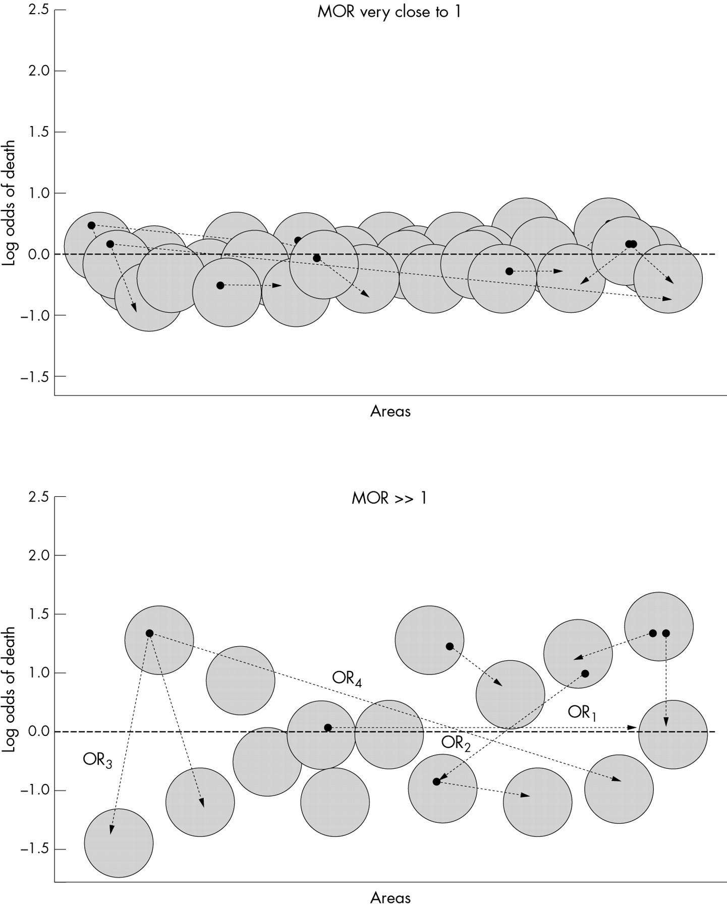
Heterogeneity between areas in the utilisation of private health care providers as expressed using the median odds ratio (MOR) computed from the empty multilevel logistic model. Two fictive cases are presented in the figure. In the top part of the figure we present a situation with very weak variations between areas. In the bottom part of the figure, area level variations were much stronger, which will be reflected in a higher MOR. Considering the area level residuals of the multilevel model, the odds ratio between the person at lowest risk and the person at highest risk is computed for each pair of persons from different areas. Four arbitary comparisons (R1, R2, R3, R4) are represented in the bottom part of the figure. The MOR is defined as the median value of the distribution of this odds ratio (see fig 2). (Observe that for reasons of simplicity we have not represented all the arrows for the comparisons).

Considering the area level residuals of the multilevel model, we computed the odds ratio between the person at lowest risk and the individual at highest risk for each pair of persons from different areas. We present the distribution of this odds ratio for the 56 million pairs of persons from different areas that can be formed in our sample of 10 723 people. As shown in the figure, the MOR is defined as the median value of the distribution. Practically the MOR is very easy to calculate (see formula 6 in the text).
In practice, it is not necessary to empirically consider all possible pairs of persons from different areas. The MOR depends directly on the area level variance and can be computed with the following formula:

where VA is the area level variance, and 0.6745 is the 75th centile of the cumulative distribution function of the normal distribution with mean 0 and variance 1. See elsewhere for a more detailed explanation.8,9
If the MOR was equal to one, there would be no differences between areas in the probability of seeking a private physician (as in the fictive case presented in figure 1A). If there were strong area level differences (as in figure 1B), the MOR would be large and the area of residence would be relevant for understanding variations of the individual probability of visiting a private physician.
The standard error of the area level variance indicates the precision of the estimate. Also, using the MCMC method available in MLwiN12 and other software, we can directly compute a 95% credible interval (CrI) for the MOR using the posterior distribution of the area variance and compute the MOR for the 2.5th and 97.5th centiles of the resulting distribution. This apparently complicated technique is easy to apply use standard procedures in MLwiN software. In our example the MOR was equal to 1.81 in the empty model, with a 95%CrI (1.62 to 2.06) that clearly excluded the value 1 (table 2).
Measures of association between individual and area characteristics and the outcome and measures of variation and clustering in the utilisation of private providers in the county of Scania, Sweden, 2000, obtained from multilevel logistic models*
One feature of interest of the MOR is that it is directly comparable with the ORs of individual or area variables. In the model including individual level variables (table 2) the MOR was equal to 1.80, which shows that in the median case the residual heterogeneity between areas increased by 1.8 times the individual odds of seeking a private physician when randomly picking out two persons in different areas—that is, if a person moves to another area with a higher probability of seeking a private physician, their risk of seeking a private physician will (in median) increase 1.8 times. The residual heterogeneity between areas (MOR = 1.80) was of greater relevance than was the impact of the person’s level of education (OR = 1.25) for understanding variations in the odds of seeking a primary care physician.†
As both the MOR and the ICC are a function of the area level variance they are closely related. The epidemiologist needs to learn the meaning of the different values. For example, a small values of the area level variance (that is, = 0.04) corresponds to a MOR = 1.2 and an ICC = 1%.
About the use of the median odds ratio or the intraclass correlation coefficient for comparisons between studies with outcomes that present different prevalence. A short comment
Consider the empty model. In this model, the MOR can take any value from one to infinity for all values of the prevalence of the outcome. The ICC can also vary freely from zero to one for any prevalence of the outcome. So, in this sense, neither the MOR nor the ICC depends on the prevalence.
As MOR is a function only of the cluster variance, and ICC is a function of both the cluster variance and the individual residual variance, they are not equivalent (one to one), and therefore they measure different aspects. This is, of course, also one of the lessons that can be learned from table 1, where one can see that with a constant area variance (that is, with a constant MOR), the ICC varies as a function of the prevalence. A similar table could be constructed, where the ICC is constant and the area variance (or, equivalently, the MOR) would vary as a function of the prevalence. However, this observation does not lead to any answer as to which measure is the more “proper” to use when comparing heterogeneity between studies with different prevalence of the outcome. It only underlines that the two measures do not quantify the same thing.
As MOR quantifies cluster variance in terms of odds ratios, it is comparable to the fixed effects odds ratio, which is the most widely used measure of effect for dichotomous outcomes. The popularity of the fixed effects odds ratio is partly attributable to the fact that it does not depend on the marginal prevalence of the outcome. In this sense the odds ratio is the “canonical” choice of measure of association between explanatory variables and a dichotomous outcome. Being an odds ratio measure, the MOR inherits this property, making it as natural a measure of association between a cluster variable and a dichotomous outcome as the odds ratio in a two by two table. Consequently the MOR may be used for comparisons between studies with different prevalence.
Taking area level variance into account when interpreting associations between area variables and health with the interval odds ratio
In multilevel models regression coefficients are adjusted for the dependence of the outcome within areas by including the area level residuals in the equation (equations 1, 3, and 4). The regression coefficients for individual variables, in being adjusted for area level residuals, reflect the association between the individual level variables and the outcome within a specific area (and are termed “area specific coefficients” or “cluster specific coefficients”). However, for area variables, regression coefficients cannot be interpreted as being area specific in the same way as with individual variables: as area variables only take one value in each area it is necessary to compare persons with different area level residuals to quantify the area level effect.
In our data we found that living in areas with a high percentage of highly educated people increased the individual probability of visiting a private physician. However, if residual variability between areas remains strong, the likelihood is high of finding a person in a low education area who presents higher odds of consulting private providers than a person in a highly educated area. It is therefore particularly useful to consider the magnitude of area level residual variations when interpreting effects of area level variables. To integrate the area level fixed effect and the random residual variations we suggest using the 80% interval odds ratio (IOR-80), as described in detail elsewhere.8,9 As indicated in the two contrasted fictive cases in figure 3, the usual OR consists in comparing the mean odds in low and high education areas. By contrast, when comparing persons in areas with low education with persons in areas with high education, the IOR also takes into account the specific area level residuals.
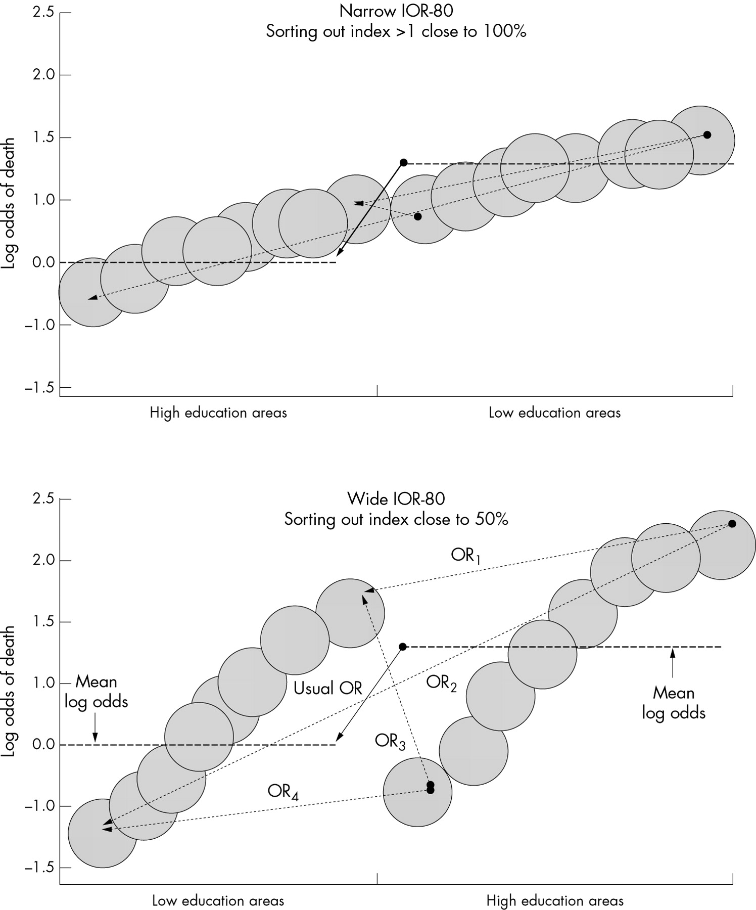
Illustration of the rationale of the interval odds ratio and of the sorting out index (that is, percentage of ORs>1). Low education areas are grouped on the left and high education areas on the right. The thick dotted black lines represent the mean odds of consulting private providers in low education and high education areas. The log odds of consulting private providers in each of the areas are function of the area educational level and of the area level residual, and are represented as grey circles over and above the thick dotted black lines. The common odds ratio consists in comparing the thick dotted black lines (see the thick black arrow). By contrast, the interval odds ratio also takes into consideration the unexplained area level variation, and therefore compares one person selected from a low education area and one person from a high education area (dotted arrows). We present two contrasted fictive cases. In the top part we present a situation in which area level residual variations are weak compared with the effect of the area educational level. Therefore, the IOR-80 is narrow and the sorting out index 1 is close to 100%. Conversely, in the bottom part, the area level variations are much stronger than the area educational effect. In that case, the likelihood is high of finding a person in a low education area who presents higher odds of consulting private providers than does a person in a highly educated area. For this reason the IOR-80 is wide and the sorting out index is close to 50%. (Observe that for reasons of simplicity we have not represented all the arrows for the comparisons).
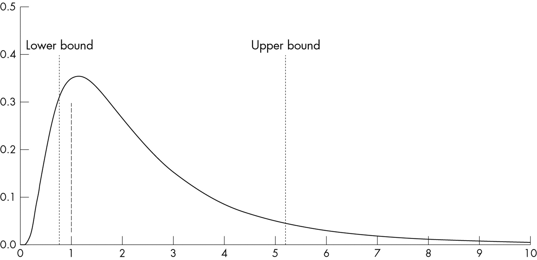
Imagine we consider all possible pairs of persons with similar covariates, in which one person resides in a low education area and the other in a high education area. For each pair, taking into account the educational level and the residual of these areas, we compute the OR between the person in the low education area and the person in the high education area (the latter person is always taken into account in the numerator of the OR, which may therefore be inferior or superior to one). Considering all possible pairs, we then obtain the distribution of this OR. The IOR-80 is defined as the interval centred on the median of the distribution that comprises 80% of the values of the OR. In figure 4 we present the distribution of the OR for the area educational level in our empirical example, and give the lower and upper bounds of the IOR.
Computation of the interval odds ratio (IOR) for the impact of the area educational variable on the utilisation of private providers (continuation of fig 3). We consider all possible pairs of persons with similar individual covariates, in which one person resides in a low education area and the other in a high education area. For each pair, taking into account the educational level and the residual of these areas, we compute the odds ratio between the person in the low education area and the person in the high education area (the latter person is always taken into account in the numerator of the odds ratio). Considering all possible pairs of persons from a low and from a high education area in our sample, we obtain the distribution of the odds ratio shown in the figure. The IOR is defined as the interval centred on the median of the distribution that comprises 80% of the values of the odds ratio. In the figure we give the lower and upper bounds of the IOR.
In practice, it is not necessary to calculate the OR for each possible pair. Rather, the lower and upper bounds of the IOR can be computed with the following equations:


where β is the regression coefficient for the area level variable, VA is the area level variance, and the values –1.2816 and +1.2816 are the 10th and 90th centiles of the normal distribution with mean 0 and variance 1. See elsewhere8,9 for more information.
The IOR-80 is not a common confidence interval. The interval is narrow if the residual variation between areas is small (fig 3, top), and wide if the variation between areas is large (fig 3, bottom). If the interval contains the value one, this indicates that the effect of the area characteristic under scrutiny is not that strong when compared with the remaining residual area level heterogeneity.
In our case, persons residing in high compared with low education areas had higher odds of visiting private physicians (OR = 1.95, 95% CI: 1.45 to 2.62). However, the IOR-80 was fairly wide (0.75 to 5.05) and comprised the value one (fig 4). In other words, in comparison with residual area level variations, the educational variable was not that important for understanding area level variations in the individual propensity for seeking a private practitioner. The IOR therefore brings complementary information to the information provided by the usual OR.
The choosing of the 80% interval is arbitrary; we could choose other intervals (for example, 70%, 90%). Also, a useful alternative measure is the percentage of ORs that are above 1. This sorting out index reports the percentage of pairs of persons in the distribution for which the odds ratio is superior to 119 (when always comparing a person with a higher propensity in the exposed category—area low education—to a person with a lower propensity in the reference category—area high education—). If the area residual variance is high and the area variable irrelevant the composite odds ratio for the area effect would only be superior to 1 in half of the cases and inferior to 1 in the other half of the cases. Conversely, if the area variable were absolutely overwhelming in comparison with residual area variance (that is, a strong of the area variable and area residual variance close to zero), the composite odds ratio would be superior to 1 in 100% of all cases. Thus, the values of the sorting out index extend between 50% and 100%. This information can be used as an informative index that indicates the extent to which the area variable under study is of importance as compared with residual neighbourhood variations.
The formula to calculate sorting out index (that is, the percentage of ORs>1) is using previous notation

For a categorical area variable with a reference category equal to 0 the equation 9 is reduced to
The Φ represents the cumulative distribution function for the normal distribution with mean zero and variance one. In practice one calculates the value of Φ for

in a table or using and excel sheet. This value can, in turn, be expressed as the percentage of pairs of persons in the distribution for which the odds ratio is superior to one. For example, if

= 0.0 the value of Φ = 0.50 and the sorting out index = 50%. If

= 1.9, the value of Φ = 0.97 and the sorting out index = 97%.
Observe that the above explained measures can be calculated in models adjusting simultaneously for several contextual factors. In our example we present only one contextual variable for reasons of simplicity.
The proportional change in variance
The percentage of proportional change in variance (PCV) concept has been discussed in detail in a related publication within this series of papers,4 and we refer the reader to these publications for further details.
In few words the PCV is calculated as

where VA = variance of the initial model, and VB = variance of the model with more terms.
DISCUSSION
We followed a didactic example on health care utilisation in Sweden to show how to calculate and interpret several measures of variance that are appropriate for investigating contextual phenomena of a binary nature. These measures provide different and complementary information. For example, the interval odds ratio is not better than the median odds ratio; they simply provide different information useful in contextual analyses.
Measuring clustering of binary phenomena within areas is certainly more problematic than measuring clustering in the linear case. Different methods have been developed to calculate the ICC in logistic models.6,7 However, the simulation method leads to ICCs that are statistically on the prevalence of the outcome, and can therefore not be used to compare the magnitude of clustering between phenomena with a different prevalence. On the other hand, the threshold method for computing the ICC necessitates conversion of binary outcomes into continuous linear latent variables, which may not be adequate for all phenomena. Furthermore, these methods for calculating the ICC in logistic regression have interpretative drawbacks when it comes to measuring clustering of phenomena, because of the inherent difficulty of distinguishing the individual level and the area level variance in the logistic case.6,8
Computing the MOR is an epidemiologically more suitable option for obtaining measures of variance in logistic regression. It is not statistically dependent on the prevalence of the outcome and furthermore permits expression of the area level variance on the well known OR scale. Therefore, it permits comparison of the magnitude of area level variations with the impact of specific factors.8,9
As previously discussed,1,5 it is useful to take into account the magnitude of residual variance between areas when interpreting associations between contextual factors and the outcome. In multilevel logistic models this information is conveyed by the IOR and the sorting out index, which indicates whether the contextual factor is useful to identify high risk areas, or whether area level variations are too strong to use the contextual factor in distinguishing high risk from low risk areas.
CONCLUSION
As previously indicated,1,5 strategies of disease prevention need to combine a person centred approach with approaches aimed at changing the residential environment.20 To gather information on cross level causal pathways, which are useful in implementing these interventions, it is relevant to investigate traditional measures of association between area socioeconomic characteristics and individual health. However, for assessing the public health relevance of specific geographical units (for example, neighbourhoods, municipalities, or districts),2 multilevel measures of health variation present themselves as the appropriate epidemiological approach in social epidemiology.
REFERENCES
Footnotes
-
↵* This parameter represents the shrunken difference between the overall prevalence on the logistic scale and the prevalence in a given area on the logistic scale. In multilevel regression analysis, the area level residuals are “shrunken” towards their mean of 0, in an attempt to disentangle the part of the variations that may be attributable to true variations between areas from that part that might be better attributed to random variations. More detailed explanations are provided in a previous paper.3
-
↵† When comparing two ORs fro two different variables one should use the same categorisation (for example, quartiles or median). In the present case the effect of individual education is a mean contrast between two groups (people with low compared with people with high educational achievement). Conversely, the MOR is the median in a distribution of contrast between pairwise neighbourhood comparisons. Therefore, the conclusion that the residual heterogeneity between areas was of greater relevance than the effect of individual education needs be interpreted with within this framework.
-
Funding: this study is supported by grants from the Swedish council for working life and social research (FAS) (PI Juan Merlo, Dnr: 2003 – 0580), the Swedish Research Council (VR) (PI Juan Merlo, Dnr 2004-6155), Region Skåne and the NEPI foundation.
-
Competing interests: none declared.
Linked Articles
- In this issue